A. S. Al-Fhaid
Department of Mathematics, College of Sciences, P.O.Box 80203 King Abdulaziz University, Jeddah - 21589, Saudi Arabia.
DOI : http://dx.doi.org/10.13005/msri/070111
Article Publishing History
Article Received on : 26 Mar 2010
Article Accepted on : 28 Apr 2010
Article Published :
Plagiarism Check: No
Article Metrics
ABSTRACT:
We consider the parabolic integrodifferential equations of a form given below. We establish local existence and uniqueness and prove the convergence in L2(En) to the solution Ut of the Cauchy problem.
KEYWORDS:
Cauchy; Parabolic; Integrodiffrential equationss; Operator
Copy the following to cite this article:
AL-FHAID A. S. Some Study of a Cauchy Problem in Parabolic Integrodifferential Equations Class. Mat.Sci.Res.India;7(1)
|
Introduction
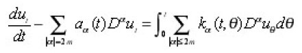
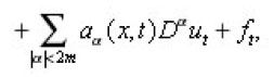
Let’s have the parabolic integrodifferential equations of the form
where the partial differential operator

is uniformly elliptic,
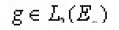
is a family of linear bounded operators defined on the space of all square integrable functions L2(En) and En is the n- dimensional Euclidean space.
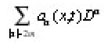
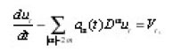
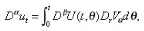
We consider integrodifferential equations of the form;
Where,
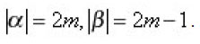
is an n-dimensional multi index,
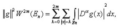
is an element of the n-dimensional Euclidean space En. Let L2(En) be the space of all square integrable function on En and Wm(En) the Sobolev space, [ the space of all functions
such that he distributional derivative

with

all belong to
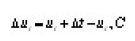
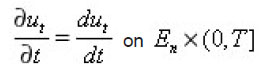
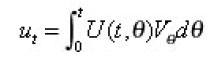
We assume that ut satisfy the Cauchy condition;
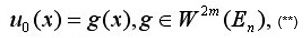
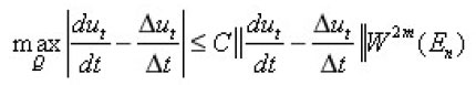
We can assume that on g(x)=0 on En. We shall say that ut is of the class S if for each

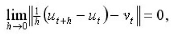
where

is the abstract derivative of ut in L2(En) in other word there is and element

such that
Where

is the norm in
Notice that if
for each
then the partial derivative

exists in the usual sense

and

in fact according to the embedding theorem [3], [8], we have
Where
is a positive constant,
is the volume enclosed by the sphere
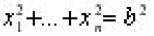
letting

we get

on Q x (0, T)
Since b is arbitrary, it follows that
Let us suppose that the following assumptions are satisfied;
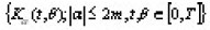
The coefficients

are real functions of t, defined on [o,T] and having continuous derivatives

on [o, T]
The deferential operator
is uniformly elliptic on [o, T]
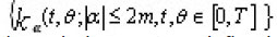
The kernels
are linear bounded operators acting on into it self. It is assumed that these operators are continuous in
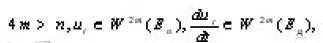
Furthermore it is assumed that the (abstract) partial derivatives

exist for all

and represents linear bounded operators on L2(En) which are continuous in
The coefficients

are real functions, which are continuous and bounded on


is a map from [0,T] into which is continuous in t with respect to the norm in

All the coefficients
have continuous bounded partial derivatives

The range of the operators
is the space

we assume that all the operators

are bounded, and that
exist for all

The operators
are supposed to be bounded and continuous in

for all

It is supposed also that

are continuous in

Proposition 1.
Under conditions (a) , …. , (e) if there is at least one solution in the class S of the Cauchy problem (*), (**), then this solution is the unique such solution.
Proof.
If
then we have the following representation:
Where
is the singular integral operator defined to be the

and
Notice that
are bounded operators from L2(En) into itself, [1],[2].
Let H1(t) be an operator defined by
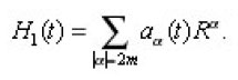
According to assumption, the operator H1(t) has a bounded inverse

defined on for every
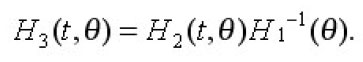
Set
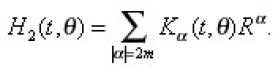
and
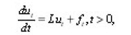
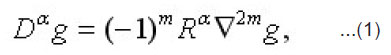
Using (1), then equation (*) can be written in the form;
To Prove the uniqueness of the considered Cauchy problem, we set
Now set
Then according to assumptions (1) and (2), we can write
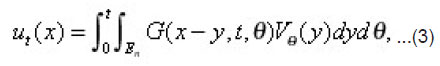
Where G is the fundamental solution of the Cauchy problem for the parabolic equation
Let
be the family of bounded operators defined by
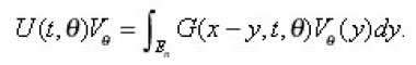
Consequently (3) can be written in the form
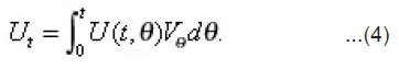
According to the well-known properties of the fundamental solution G, [4], [5], we can see that
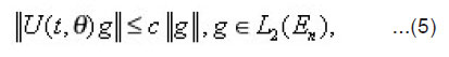
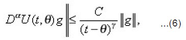
For
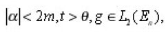
where C is a positive constant and is a constant satisfying 0<y<1. Substituting from (4) into (2), we get
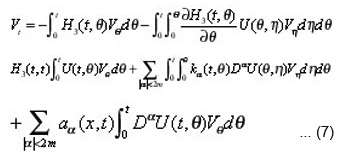
Using (5) and (6), we get from (7), the following estimation;
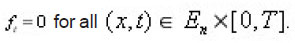
(To obtain (7) and (8), we already used conditions (c) and (d) where C is a positive constant. Thus (4) and (8) lead immediately to the fact that ut(x)=0 on E x [0,T].
Proposition2
Under the condition (a) , …, (h) the solution of the Cauchy problem (*) , (**) exists in the class S.
Proof
Using the conditions from (a) to (e), we obtain
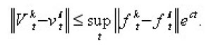
According to (5) and (6), the Volterra integral equation (9) has a unique solution t V in which satisfies:
where c is a positive constant.
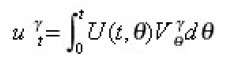
This means that under conditions from (a) to (e), we can obtain the so called mild solution [6] of the Cauchy problem (*) , (**). this solution is represented by
Now we must prove that the distributional derivatives

exists in L2(En) for all
To prove that
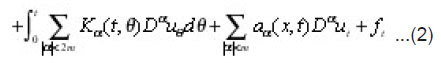
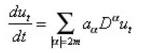
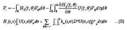
we apply formally the differential operator on both sides of the integral equation (9), then we get;
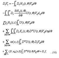
Let us consider as the unknown element in the integral equation (10). Under the assumptions (a),…, (h) this integral equation can be solved for

Thus
for
Now we have
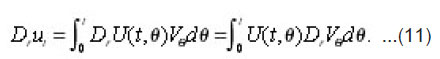
Using (11), we can wire
Where
Proposition 3
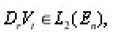
Let

L2(En) for every

and continuous in t. suppose.
Where

is continuous in

if is a sequence of functions of the class S, which are solutions of the Cauchy problem
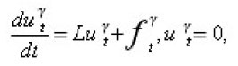
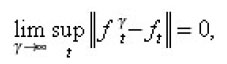
then

converges in L2(En) to the solution of the Cauchy problem (*), (**).
Proof. Set
We find
References
- A.S. Al-Fhaid, The Derivation of Interstellar Extinction Curves and Modelling, Ph.D. Thesis.
- A. S. Al-Fhaid, Continued fraction Evaluation of the Error function. To appear.
- Calderon H. P., Zygmond A. Singular Integral Operators and Differential Equations II, Amer J. Math., 79,(3); (1957).
- EhrenperiesL, Cauchy’s Problem for linear Differential Equations with constant coef-ficients II, Proc. Nat. Acad. Soi USA, 42. Nv. 9.
- El-Borai. M. On the correct formulation of the Canchy problem Vesnik Moscow univ. 4 (1968).
- Friedman A. Partial differential Equations, Robert E. Krieger Publishing Company, New York, 101-102 (1976).
- Hormander L. , Linear partial differential Operators ( Springer – Verlag) , Berlin, New York (1963).
CrossRef
- Samuel M. R., Semilinear Evolution equations in Banach spaces with applications of Parabolic partial differential Equations, Trous Amer. Math. Soc. 33: 523-535 (1993).
- Yosida K. Functional Analysis, Spreinger verlage, (1974).

This work is licensed under a Creative Commons Attribution 4.0 International License.