Group Analysis and Variational Principle for Nonlinear (3+1) Schrodinger Equation

Eman Salem A. Alaidarous

Department of Mathematics, Faculty of Science, King Abdul Aziz University, P.O. Box 80203, Jeddah 21589, Saudi Arabia.

DOI : http://dx.doi.org/10.13005/msri/070113

ABSTRACT:

The generators of the admitted variational Lie symmetry groups are derived and conservation laws for the conserved currents are obtained via Noether's theorem. Moreover, the consistency of a functional integral are derived for the nonlinear Schrödinger equation. In addition to this analysis functional integral are studied using Lie groups.

KEYWORDS: Nonlinear (3+1) schrodinger equation; Noether's theorem; Lie groups

Copy the following to cite this article: Alaidarous E. S. A. Group Analysis and Variational Principle for Nonlinear (3+1) Schrodinger Equation. Mat.Sci.Res.India;7(1)

Copy the following to cite this URL: Alaidarous E. S. A. Group Analysis and Variational Principle for Nonlinear (3+1) Schrodinger Equation. Mat.Sci.Res.India;7(1). Available from: http://www.materialsciencejournal.org/?p=2242

Introduction

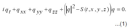
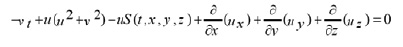
In recent years, a number of works of the symmetry methods are found to be very efficient in applications to differential equations in Physics and Engineering. A subject of a special interest is a study of invariance properties of the equations with respect to local Lie groups point transformations of dependent and independent variables. The importance of the conservation laws lies in the fact that there are situations where numerical schemes have been devised keeping in view the conservation form of the DEs. Also, the conservation law can be used for serving a priori estimates and to obtain integrals of motion, where for certain types of solutions, the conserved density, when integrated, provides us with a constant of motion of the system. Actually, finding the conservation laws of a system is often the first step towards finding its solution. Rund¹ and Logan² have studied the invariance of fundamental functional integral and deduced the first integrals or conservation law for the corresponding system of DEs. The nonlinear (3+1) Schrödinger equation [3, 4] is described by nonlinear couple partial differential equations. It is well know that a part of one parameter symmetry groups of these equations turns out to be their variational symmetries. According to Noether theorem [5, 6] such as invariance of the elementary action is a necessary and sufficient condition of the existence of conservation laws for the Schrödinger equation. Let us consider Schrödinger equation with nonlinear term:

Group Analysis

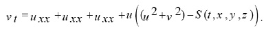
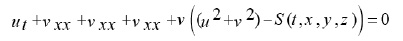
Equations (1) have some applications in quantum field theory, plasma physics and Engineering [3]. To simplify equation (1), set q =u+iv then, eq. (1) is divided into couple of equations as follows:

In order to find invariance transformations, we look for infinitesimal Lie point transformations of the form:

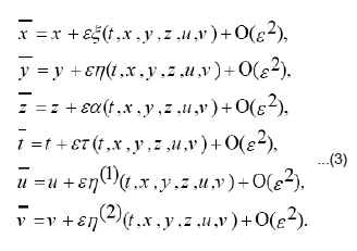
which (2-i, 2-ii) system.

Following the widely used methods in the classical monographs. Concerning these arguments [4-12] we find the coordinates

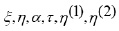
by solving over the determined linear PDE system, usually called the determining system which is obtained by requiring, the invariance of the system (2-i,2-ii) with respect to (3). (1)(2),,,,,……

There are many software packages which aid researchers in obtaining the determining system.

Then we have the following cases:

Case 1

When λ1=λ2=λ3 and Ψ=0 then the infinitesimal take the form

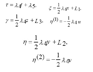
But solving it with arbitrary functions requires analysis. We omit the determining system from which we are able to obtain the following results in the form of the coordinates

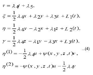
and

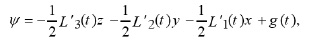
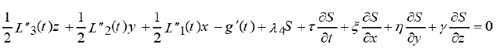
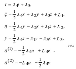
where, λ₁, λ₂, λ₃ and λ₄ arbitrary constants and L’1(t), L’2(t), L’3(t) are arbitrary functions. Let the function ) S (t, x, y, z,) satisfies the equation and ) S (t, x, y, z,) satisfies the equation:

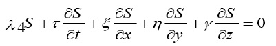
By applying the invariance surface condition, we obtain

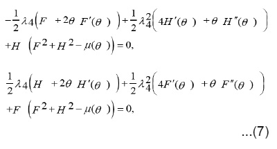
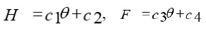
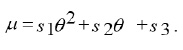
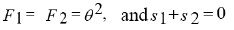
Where λ₁, λ₂, L₁, L₂ are constants and F, H, μ are functions to be determined by substituting ( 4 ) into the system (2-i,2-ii) ,that is ,by solving the following reduced system

In order to solve system (6), we change the variables

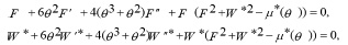
Consequently, the system (6) takes the form:

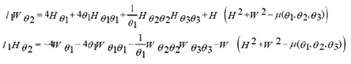
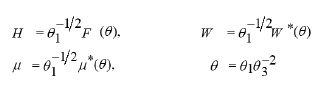
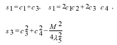
We make use of dilation group and after some manipulations on the system (10) we have

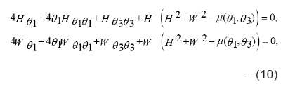
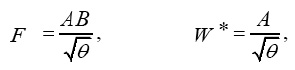
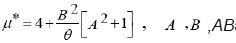
from (7), we have

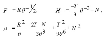
where,,TRN are constants.

Case 2
When λ4=λ3=L1=L2=L3=Ψ=0, then the infinitesimal takes the form

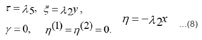
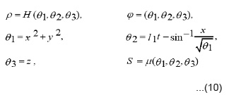
The invariance surface condition may be solved to yield the functional form:

This leads to a reduction of the system (2) in the following form

and

This leads to a reduction of the system (2) in the following form Where

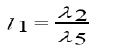
using again dilation group on the system (11) one gets

where

Consequently, system (12) has the solution

when

are constants.

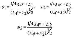
Case 3
In this case the infinitesimal takes the form

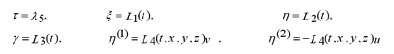
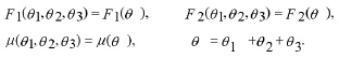
Applying the rules as before (such as case 1, 2), we get:

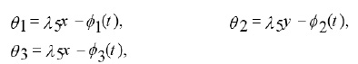
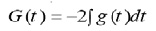
where

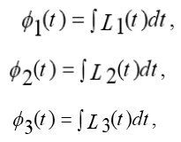
and

Hence ,

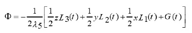
where,

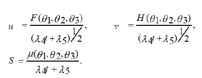
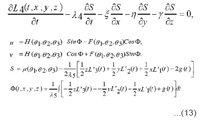
Using the transformation 

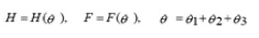
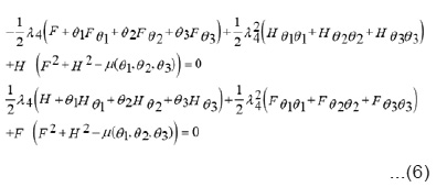
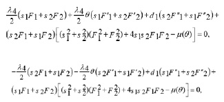
and system (13) in (2), we obtain,

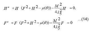
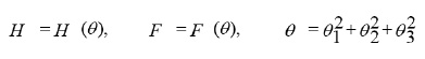
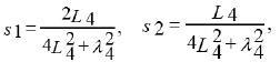
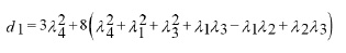
After some calculations on (14), we have the solution in the form:

provided that

where,

are constants, and

Case 4

When L1(t), L2(t), L3(t) and Ψ(t,x,y,z) are constant, we get

 and

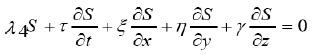
From (15), the invariance surface condition leads to:

 

and

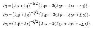
where

using (16) and changing the variables

then (2) can be written as the follows

and

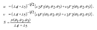
System (16) has the solution

In this case

is an arbitrary function.

Variational Principle

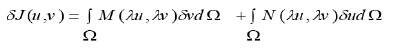
In order to study variational principle for our problem,

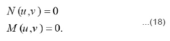
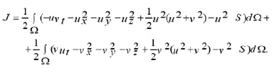
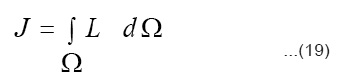
The system (18) satisfied the consistency conditions for the existence of functional integral. Consequently, a functional integral can be written by using the formula given by Tonti [8, 9] as: ),(vuJ
Since

or

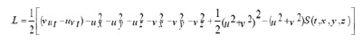
since

with L being the Lagrangian function, we obtain

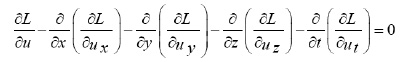
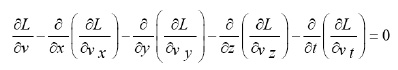
for which the Euler-Lagrange equation is

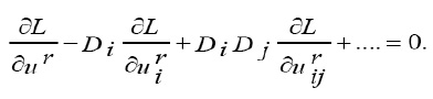
Consequently we have

Hence,

This leads to

Moreover as,

we obtain

In order to prove the invariance of the fundamental functional integral

where L is the Lagrangian function and Ω represents the domain of integration to be invariant under the one-parameter group of transformations (3), we can use the following theorem:

Theorem 1 [ 2]
If the fundamental functional integral defined by (19) is invariant under the ƒ{rparameter family of transformation (3), then the Lagrangian L and its derivatives satisfy the ƒ{ridentities:

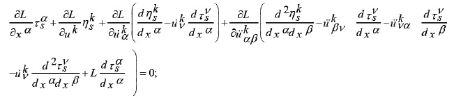
for

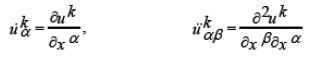
where

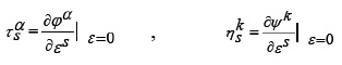
and

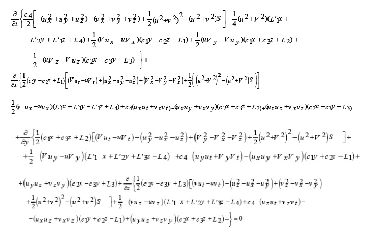
Then, Lagrangian and its derivatives must satisfy the condition: L

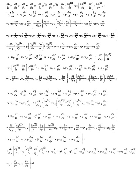
On Substituting for L and its derivatives in equation (21), we get a polynomial in

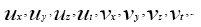
etc Collecting it in descending order of various powers of

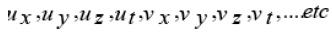
and equating to zero the different powers of

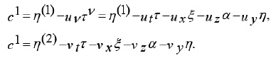
we obtain a system of first order PDEs. On solving this system, we get the following expressions for

 and n⁽²⁾

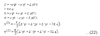
and

where c1, c2, c3 and 4c are arbitrary constants, but L1, L2, L3 and L4 and φ arbitrary functions of t[12-19].

By using the following theorem

Theorem 2

(Noether‘s Identity)[5,10] Under the hypothesis of theorem 1, the following ƒ{rconservation laws hold true

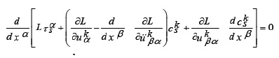
where

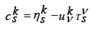
Consequently

thus , we have

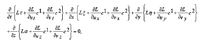
where,

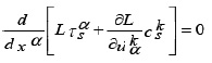
Hence

Conclusion

This paper is concerned with finding potentials that admit Lie point symmetries for the nonlinear (3+1) Schrödinger equation, i.e., we give a classification of potentials admitting point symmetries. Finally, we apply Noether’s theorem to show which of this point symmetries are variational and we obtain the corresponding conservation laws

References

1. Rund, H., The Hamilton-Jacobi theory in the calculus of variations. Princeton, NewJersy,(1966).
2. Logan,J.D., Invariant Variational Principles., Academic Press, (1977).
3. Herrera, J.J.E., J.Phys.A:Math.Gen. 17: 95-98 (1984).
4. Cupta, M.R., Physics Lett.,69(3): 172-174(1987).
5. Logan, J., A equations Math., 9: 210-220(1973).
6. Bluman, G., Symmetries and differential equation., Spinger- Ver variational principle lag, New York (1989).
7. P. J. Olver., Applications of Lie Groups to Differential Equations. Springer, New York (1986).
8. Hassan Zedan, Int,J . Non- Linear Mech.,30: 469-489 (1995).
9. Tonti,E., Acad Roy. Belg. Bull. Cl. Sci., 55:137-165 (1969).
10. Tonti,E., Acad Roy . Belg.Bull.Cl.Sci., 55: 262-278 (1969).
11. Logan,J.D.,J. Math. Anal. Appl.,.48: 618-631(1974).
12. Logan, J.D., Noether theorem and calculus of variations. Ph.D. Dissertation, Ohio State University, Columbus (1970).
13. Hassan Zedan, J.Comp. Math. Appl.,32: 1-6(1990).
14. Zayed, E.M.E., Hassan zedan, Int.J .of Nonlinear Science and Numerical Simulation, 5: 221-234 (2004).
15. Zayed, E. M. E., Hassan zedan, Chaos, Solitons and Fractal, 16: 133-145 (2003).
16. Zayed, E.M.E., Hassan zedan, Int.J. Theor. Phys., 40: 1183-1196 (2001).
17. Zayed, E.M.E., Hassan zedan, Chaos,Solitons and Fractal, 13: 331-336,(2002).
18. Zayed, E.M.E., Hassan zedan, Applicable Analysis, 83(11): 1101-1132 (2004).
19. Zayed, E.M.E., Hassan zedan, Applicable Analysis,.84(4): 1-19 (2005).

---

This work is licensed under a Creative Commons Attribution 4.0 International License.